Isolation Forestとは
Isolation Forestとは有名な異常検知手法の一つです。 Forestという名前からもわかるように決定木の仕組みを使って異常検知を行います。 ざっくりいうと決定木の早いタイミングで分類されるものは、異常である可能性が高いといった感じです。 詳細説明は参考文献にあるリンクがわかりやすいのでそちらに託します。
実装
ライブラリ準備
import numpy as np
import matplotlib.pyplot as plt
from sklearn.ensemble import IsolationForest
データ準備
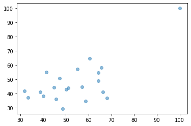
今回はダミーデータを作って検証していきます。 正規分布に基づく正常データと一つの異常データを作っています。
x_normal = np.random.normal(50, 10, 20)
x_normal = x_normal[:, np.newaxis]
y_normal = np.random.normal(50, 10, 20)
y_normal = y_normal[:, np.newaxis]
data_normal = np.concatenate([x_normal, y_normal], axis=1)
data_abnormal = np.array([100, 100])
data_abnormal = data_abnormal[np.newaxis, :]
data = np.concatenate([data_normal, data_abnormal])
plt.scatter(data[:, 0], data[:, 1], alpha=0.5)
plt.show()
plt.clf()
IsolationForest
それではIsolationForestで実装します。
clf = IsolationForest(random_state=0)
clf.fit(data)
predict = clf.predict(data)

predict_normal = data[np.where(predict==1)]
predict_abnormal = data[np.where(predict==-1)]
plt.scatter(predict_normal[:, 0], predict_normal[:, 1], alpha=0.5, label="predict_normal")
plt.scatter(predict_abnormal[:, 0], predict_abnormal[:, 1], alpha=0.5, label="predict_abnormal")
plt.legend()
plt.show()
plt.clf()
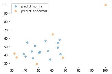
はい、できました。 これを見ると想定していない点まで異常値となってしまっていますね。
これを回避するにはclf.predict(data)ではなく、clf.decision_function(data)を使いましょう。
下の結果を見るとわかるようにpredictのデフォルトでは、decision_functionで予測された値の正負によって異常値かどうかを判断しています。
なのでdecision_functionで予測させたのちに任意の閾値を設定することで想定している異常値だけを取得できることになります。
print(clf.predict(data))
"""出力結果
array([-1,  1,  1,  1,  1, -1,  1,  1,  1,  1,  1, -1,  1,  1,  1,  1,  1,
        1,  1, -1, -1])
"""
print(clf.decision_function(data))
"""出力結果
array([-0.00135646,  0.08005558,  0.1082589 ,  0.00546616,  0.06094732,
       -0.06203556,  0.08608974,  0.08951439,  0.0525859 ,  0.09442839,
        0.10014535, -0.04470121,  0.02635501,  0.11540577,  0.04846334,
        0.07833354,  0.09563196,  0.04730001,  0.04987712, -0.07718921,
       -0.29339037])
"""
それでは閾値を-0.1にして確認してみます。
predict = clf.decision_function(data)

threshold = -0.1
predict_normal = data[np.where(predict > threshold)]
predict_abnormal = data[np.where(predict <= threshold)]
plt.scatter(predict_normal[:, 0], predict_normal[:, 1], alpha=0.5, label="predict_normal")
plt.scatter(predict_abnormal[:, 0], predict_abnormal[:, 1], alpha=0.5, label="predict_abnormal")
plt.legend()
plt.show()
plt.clf()
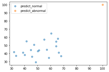
はい、できてますね。
可視化
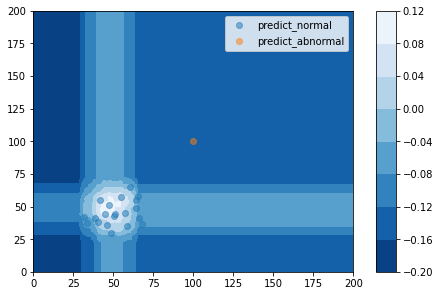
次に異常値の領域を可視化してみましょう。
# データ準備
xx, yy = np.meshgrid(np.linspace(0, 200, 400), np.linspace(0, 200, 400))
mesh_predict = clf.decision_function(np.c_[xx.ravel(), yy.ravel()])
mesh_predict = mesh_predict.reshape(xx.shape)

# 可視化
fig1, ax2 = plt.subplots(constrained_layout=True)
CS = ax2.contourf(xx, yy, mesh_predict, cmap=plt.cm.Blues_r)

ax2.scatter(predict_normal[:, 0], predict_normal[:, 1], alpha=0.5, label="predict_normal")
ax2.scatter(predict_abnormal[:, 0], predict_abnormal[:, 1], alpha=0.5, label="predict_abnormal")
ax2.legend()

cbar = fig1.colorbar(CS)
以上です。