概要
この記事ではpythonを使ってX-means法を実装していきます。ライブラリはpyclusteringを用いています。
X-means法とは
X-means法とはクラスタリング手法の一つです。k-means法の改良版であり、その特徴は初めにクラスタ数を決める必要がないということです。なのでクラスタ数が未知の場合において、最適なクラス多数を探し出しクラスタリングをしてくれます。
実装
それでは実装に移ります。今回は
- 1次元データ
- 2次元データ
の2種類のデータに対して実装していきます。
1次元データ
はじめにライブラリをインポートします。
import numpy as np
import pandas as pd
import matplotlib.pyplot as plt
from sklearn import cluster, preprocessing
from pyclustering.cluster.xmeans import xmeans
from pyclustering.cluster.center_initializer import kmeans_plusplus_initializer
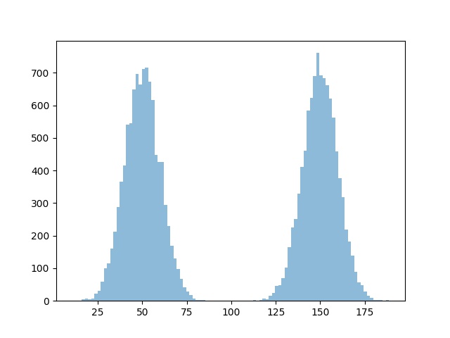
実験に使うデータを用意します。今回は平均50, 標準偏差10のx_1と平均150, 標準偏差10のx_2の二つのデータを用意します。
x_1 = np.random.normal(50, 10, 10000)
x_2 = np.random.normal(150, 10, 10000)
x = np.concatenate([x_1, x_2])
x = x.reshape([x.shape[0], 1])

# 描画
plt.hist(x, bins=100, alpha=0.5)
plt.savefig("xmeans_sample1.jpg")
plt.clf()
データが用意できたので早速クラスタリングしていきます。
xm_c = kmeans_plusplus_initializer(x, 2).initialize()
xm_i = xmeans(data=x, initial_centers=xm_c, kmax=20, ccore=True)
xm_i.process()
結果の確認をしていきましょう。
classes = len(xm_i._xmeans__centers)
predict = xm_i.predict(x)

for i in range(classes):
    batch_predict = x[predict==i]
    n, _, _ = plt.hist(batch_predict, bins=100, alpha=0.5, label="class="+str(i))
    plt.vlines(xm_i._xmeans__centers[i], 0, max(n))

plt.legend()
plt.savefig("xmeans_result1.jpg")
plt.clf()
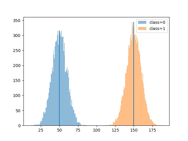
2つのクラスにクラスタリングできてそうですね。centroidもそれぞれの平均値にかなり近くなっています。
2次元データ
続いて2次元データです。1次元と同様にライブラリのインポートを行います。
import numpy as np
import pandas as pd
import matplotlib.pyplot as plt
from sklearn import cluster, preprocessing
from pyclustering.cluster.xmeans import xmeans
from pyclustering.cluster.center_initializer import kmeans_plusplus_initializer
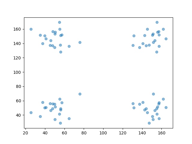
データの用意です。今回は4つのクラスを想定しています。
x_1 = np.random.normal(50, 10, 20)
x_1 = x_1.reshape([x_1.shape[0], 1])
x_2 = np.random.normal(150, 10, 20)
x_2 = x_2.reshape([x_2.shape[0], 1])
y_1 = np.random.normal(50, 10, 20)
y_1 = y_1.reshape([y_1.shape[0], 1])
y_2 = np.random.normal(150, 10, 20)
y_2 = y_2.reshape([y_2.shape[0], 1])

data1 = np.concatenate([x_1, y_1], axis=1)
data2 = np.concatenate([x_1, y_2], axis=1)
data3 = np.concatenate([x_2, y_1], axis=1)
data4 = np.concatenate([x_2, y_2], axis=1)
x = np.concatenate([data1, data2, data3, data4])

plt.scatter(x[:, 0], x[:, 1], alpha=0.5)
plt.savefig("xmeans_sample2.jpg")
plt.clf()
それではデータが用意できたので同様にクラスタリングしていきます。特に1次元の時と変更はなしです。
xm_c = kmeans_plusplus_initializer(x, 2).initialize()
xm_i = xmeans(data=x, initial_centers=xm_c, kmax=20, ccore=True)
xm_i.process()
結果を確認します。
classes = len(xm_i._xmeans__centers)
predict = xm_i.predict(x)

for i in range(classes):
    batch_predict = x[predict==i]
    plt.scatter(batch_predict[:, 0], batch_predict[:, 1], alpha=0.5, label="class="+str(i))

centers = np.array(xm_i._xmeans__centers)
plt.scatter(centers[:, 0], centers[:, 1], label="centroids", marker='*', color="red")

plt.legend()
plt.savefig("xmeans_result2.jpg")
plt.clf()

しっかり4つにクラスタリングされてますね!
最後に
pyclusteringを使ってX-means法を動かしてみた。