概要
今回紹介するnotebookはNatural Language Processing (NLP) 🧾 for Beginnersです。 この記事は自然言語処理初学者向けであり、自然言語処理に関する概念や自然言語処理と機械学習をどのように組み合わせるのかについて主に書かれています。 それでは早速みていきましょう!
内容
目次
- テキストを数値データとして表現する
- テキストベースのデータをpandasで読み込む
- 探索的データ分析(EDA)
- テキスト前処理
- モデルの構築と評価
import pandas as pd
import numpy as np
import matplotlib.pyplot as plt
import seaborn as sns

%matplotlib inline
sns.set_style("whitegrid")
plt.style.use("fivethirtyeight")
テキストを数値データとして表現する
# サンプルで使う文章を用意
simple_train = ['call you tonight', 'Call me a cab', 'Please call me... PLEASE!']
Text Analysis is a major application field for machine learning algorithms. However the raw data, a sequence of symbols cannot be fed directly to the algorithms themselves as most of them expect numerical feature vectors with a fixed size rather than the raw text documents with variable length.
要するに生のテキストデータではそのまま機械学習のアルゴリズムに適用できないので、数値データに変換しましょうねー、ということです。
今回はいくつかある数値データへの変換手法の中の、CountVectorizerを使います。これはテキストデータを単語の頻出度合のベクトルに変換する処理のことです。少しわかりにくいですが実際コードを触りながら確認してみましょう。
# CountVectorizerの初期化
from sklearn.feature_extraction.text import CountVectorizer
vect = CountVectorizer()
# 文章に出てくる単語を辞書化する。語彙を学習するという。
vect.fit(simple_train)
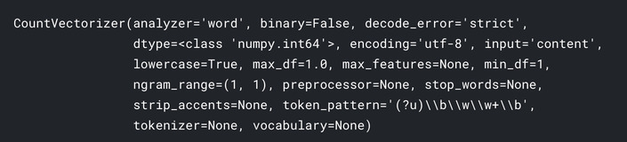
# 学習した語彙を確認する。
vect.get_feature_names()

# 学習モデルを用いてサンプルデータを変換する
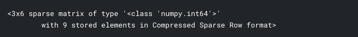
simple_train_dtm = vect.transform(simple_train)
simple_train_dtm
# 配列に変換
simple_train_dtm.toarray()
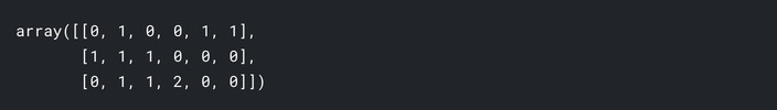
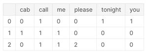
# 単語と配列を確認する。文章ごとに単語が出てきた頻度が格納されてます
pd.DataFrame(simple_train_dtm.toarray(), columns=vect.get_feature_names())
# 型確認
type(simple_train_dtm)

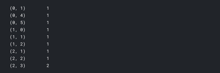
# sparseの中身
print(simple_train_dtm)
scikit-learnのドキュメントによると
As most documents will typically use a very small subset of the words used in the corpus, the resulting matrix will have many feature values that are zeros (typically more than 99% of them).
For instance, a collection of 10,000 short text documents (such as emails) will use a vocabulary with a size in the order of 100,000 unique words in total while each document will use 100 to 1000 unique words individually.
In order to be able to store such a matrix in memory but also to speed up operations, implementations will typically use a sparse representation such as the implementations available in the scipy.sparse package.
要するに文章が長くなるほどユニークな単語が増えていき、特徴量の数が膨大になっていきます。それをscipy.sparseを利用してスパース表現して、メモリの格納や操作の高速化を行っているとのこと。(多分)
# テストデータのサンプルを作って試してみましょう。
simple_test = ["please don't call me"]
simple_test_dtm = vect.transform(simple_test)
simple_test_dtm.toarray()

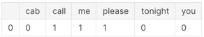
# 単語と配列を確認する。単語が出てきた頻度が格納されてます
pd.DataFrame(simple_test_dtm.toarray(), columns=vect.get_feature_names())
テキストベースのデータをpandasで読み込む
ここからKaggleにあるデータセットを用いて処理を確認していきます。 ここではSMS Spam Collection Datasetを利用します。
# csvのパスはそれぞれの環境に合わせてください
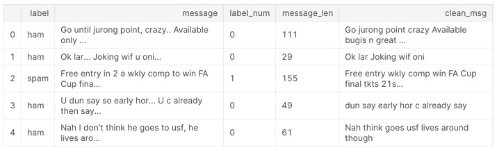
sms = pd.read_csv("/kaggle/input/sms-spam-collection-dataset/spam.csv", encoding='latin-1')
sms.dropna(how="any", inplace=True, axis=1) # ここでは欠損値は削除しているみたい
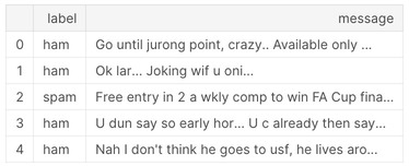
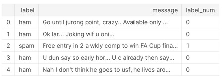
sms.columns = ['label', 'message']
sms.head()
探索的データ分析(EDA)
# 各項目における基本情報をざっと見れるので便利
sms.describe()

# ラベルごとの基本情報をみることができる
sms.groupby('label').describe()
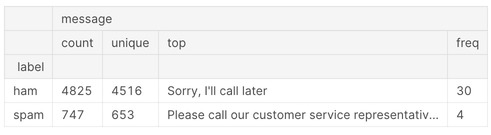
上記より、hamが4825、spamが747と少し偏りがあることがわかります。
# ラベルデータを数値に変換
sms['label_num'] = sms.label.map({'ham':0, 'spam':1})
sms.head()
分析をしていく中で実際に学習の際に用いる特徴量を意識することはとても重要です。 これは自然言語処理に関わらず一般的に重要な考えになります。
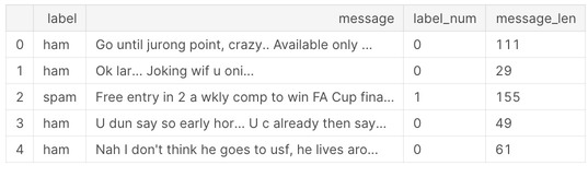
# 文章の長さについて見ていきます
sms['message_len'] = sms.message.apply(len)
sms.head()
plt.figure(figsize=(12, 8))

sms[sms.label=='ham'].message_len.plot(bins=35, kind='hist', color='blue',
                                       label='Ham messages', alpha=0.6)
sms[sms.label=='spam'].message_len.plot(kind='hist', color='red',
                                       label='Spam messages', alpha=0.6)
plt.legend()
plt.xlabel("Message Length")
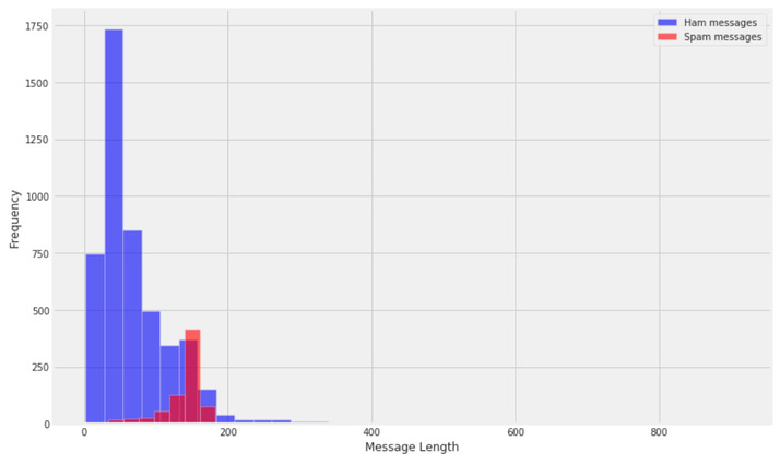
基本的なことを行うだけでもこのように傾向を掴むことができるので、EDAはやはり大切。
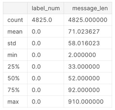
# ハムのデータ概要
sms[sms.label=='ham'].describe()
# スパムのデータ概要
sms[sms.label=='spam'].describe()
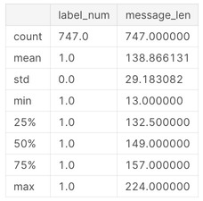
最大で910もの長さの文章がありますね。 少しこのデータを覗いてみましょう。
sms[sms.message_len == 910].message.iloc[0]

テキスト前処理
テキストの前処理の主な目的はテキストデータを数値データに変換することです。 数値データに変換することで、一般的に使われる分類アルゴリズムを使うことができるようになります。
Tokenization(トークン化)
最初のステップとして、文章を個々の単語に分割してリストを返す関数を作成しましょう。 またはじめに一般的な単語(「the」、「a」など)も削除します。 これを行うには、nltkを利用します。 nltkはテキスト処理するためのPythonの標準ライブラリであり、多くの便利な機能を備えています。 ここでは、基本的な一部の機能を使用します。 (いつかnltkの使い方についてもまとめたい)
それでは処理関数を作っていきます。
import string
from nltk.corpus import stopwords

def text_process(mess):
    STOPWORDS = stopwords.words('english') + ['u', 'ü', 'ur', '4', '2', 'im', 'dont', 'doin', 'ure']
    nopunc = [char for char in mess if char not in string.punctuation]
    nopunc = ''.join(nopunc)
    return ' '.join([word for word in nopunc.split() if word.lower() not in STOPWORDS])
sms['clean_msg'] = sms.message.apply(text_process)
sms.head()
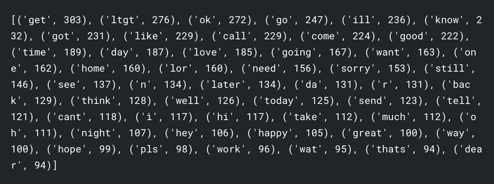
ハムとスパムの頻出単語を少し見てみましょう。
words = sms[sms.label=='ham'].clean_msg.apply(lambda x: [word.lower() for word in x.split()])
ham_words = Counter()

for msg in words:
    ham_words.update(msg)

print(ham_words.most_common(50))
words = sms[sms.label=='spam'].clean_msg.apply(lambda x: [word.lower() for word in x.split()])
spam_words = Counter()

for msg in words:
    spam_words.update(msg)

print(spam_words.most_common(50))

Vectorization(ベクトル化)
トークン化の次はベクトル化です。 ベクトル化して数値化することにより機械学習アルゴリズムを適用することができるようになります。
はじめに、トレインデータとテストデータに分けておきましょう。
from sklearn.model_selection import train_test_split

X = sms.clean_msg
y = sms.label_num

X_train, X_test, y_train, y_test = train_test_split(X, y, random_state=1)
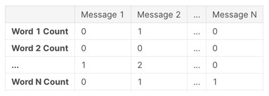
続いて文章ごとで出てくる単語のカウントをしていきます。
イメージは以下の図です。
文章と単語のマトリクスでそれぞれの単語がどのくらいその文章で出てきたかを表します。
from sklearn.feature_extraction.text import CountVectorizer

vect = CountVectorizer()
X_train_dtm = vect.fit_transform(X_train)
X_test_dtm = vect.transform(X_test)
最後にTF-IDFを使ってベクトル化をします。 TF-IDFに関してはこちらの記事を参考にしてください。
from sklearn.feature_extraction.text import TfidfTransformer

tfidf_transformer = TfidfTransformer()
tfidf_transformer.fit(X_train_dtm)
tfidf_transformer.transform(X_train_dtm)
モデルの構築と評価
それではモデルを構築していきます。
ナイーブベイズ分類
今回はナイーブベイズ分類を用います。
from sklearn.naive_bayes import MultinomialNB
nb = MultinomialNB()
nb.fit(X_train_dtm, y_train)
テストデータで予測
y_pred_class = nb.predict(X_test_dtm)
Accuracyでモデルを評価
from sklearn import metrics
metrics.accuracy_score(y_test, y_pred_class)

混同行列。
metrics.confusion_matrix(y_test, y_pred_class)
Pipeline処理
前処理を行って機械学習アルゴリズムを適用してと、いちいち処理を記述していくのは少しめんどくさいです。 そこでPipelineを作成してそれをひとまとめにしていくと楽チンです。
from sklearn.feature_extraction.text import TfidfTransformer
from sklearn.pipeline import Pipeline

pipe = Pipeline([('bow', CountVectorizer()),
                 ('tfid', TfidfTransformer()),
                 ('model', MultinomialNB())])

pipe.fit(X_train, y_train)

y_pred = pipe.predict(X_test)